This vignette demonstrates how to use this package to generate different types of html reports that allow you to visually review multiple related time series quickly and easily.
Data format
The data frame containing the time series should be in long format, with the following columns (though the actual column names can be different):
- one “timepoint” (date/posixt) column which will be used for the x-axes. Values should follow a regular pattern, e.g. daily or monthly, but do not have to be consecutive.
- one or more “item” (character) columns containing categorical values identifying distinct time series.
- one “value” (numeric) column containing the time series values which will be used for the y-axes.
Example:
The example_prescription_numbers dataset is provided
with this package, and contains (synthetic) examples of aggregate
numbers of antibiotic prescriptions given in a hospital over a period of
a year. It contains 5 columns:
- PrescriptionDate - The date the prescriptions were written
- Antibiotic - The name of the antibiotic prescribed
- Spectrum - The spectrum of activity of the antibiotic. This value is always the same for a particular antibiotic
- NumberOfPrescriptions - The number of prescriptions written for this antibiotic on this day
- Location - The hospital site where the prescription was written
# first, attach the package if you haven't already
library(mantis)

# this example data frame contains numbers of antibiotic prescriptions
# in long format
data("example_prescription_numbers")

head(example_prescription_numbers)
#> # A tibble: 6 × 5
#>   PrescriptionDate Antibiotic    Spectrum NumberOfPrescriptions Location
#>   <date>           <chr>         <chr>                    <dbl> <chr>
#> 1 2022-01-01       Coamoxiclav   Broad                       45 SITE1
#> 2 2022-01-01       Gentamicin    Broad                       34 SITE1
#> 3 2022-01-01       Ceftriaxone   Broad                       36 SITE1
#> 4 2022-01-01       Metronidazole Limited                     17 SITE1
#> 5 2022-01-01       Meropenem     Broad                       10 SITE1
#> 6 2022-01-01       Vancomycin    Limited                      0 SITE1
Specifying the data columns
You must specify which column(s) in the supplied data frame should be
used to identify the individual time series (items), and which columns
contain the timepoint (x-axis) and value (y-axis) for the time series.
These are set using the item_cols,
timepoint_col and value_col parameters of
inputspec() respectively. Any other columns in the data
frame are ignored.
Optionally, if there are multiple columns specified in
item_cols, one of them can be used to group the time series
into different tabs on the report, by using the tab_col
parameter.
Members of item_cols should be specified in the order
that you want them to appear in the output.
Example:
For the example_prescription_numbers dataset above, the
combination of “Antibiotic” and “Location” columns uniquely identify a
time series in the data frame, and so both columns must be included in
item_cols.
The “Spectrum” column can also be added to item_cols as
well if desired, in which case it will appear in the output as an
additional column/label. Otherwise it will be ignored.
Here are some options for specifying the data columns, depending on how you want the report to look:
# create a flat report, and include the "Location" and "Antibiotic" fields
# in the content
inspec_flat <- inputspec(
  timepoint_col = "PrescriptionDate",
  item_cols = c("Location", "Antibiotic"),
  value_col = "NumberOfPrescriptions",
  timepoint_unit = "day"
)

# create a flat report, and include the "Location", "Spectrum", and "Antibiotic"
# fields in the content
inspec_flat2 <- inputspec(
  timepoint_col = "PrescriptionDate",
  item_cols = c("Location", "Spectrum", "Antibiotic"),
  value_col = "NumberOfPrescriptions",
  timepoint_unit = "day"
)

# create a tabbed report, with a separate tab for each unique value of
# "Location", and include just the "Antibiotic" field in the content of each tab
inspec_tabbed <- inputspec(
  timepoint_col = "PrescriptionDate",
  item_cols = c("Antibiotic", "Location"),
  value_col = "NumberOfPrescriptions",
  tab_col = "Location",
  timepoint_unit = "day"
)

# create a tabbed report, with a separate tab for each unique value of
# "Location", and include the "Antibiotic" and "Spectrum" fields in the content
# of each tab
inspec_tabbed2 <- inputspec(
  timepoint_col = "PrescriptionDate",
  item_cols = c("Antibiotic", "Spectrum", "Location"),
  value_col = "NumberOfPrescriptions",
  tab_col = "Location",
  timepoint_unit = "day"
)

# create a tabbed report, with a separate tab for each unique value of
# "Antibiotic", and include just the "Location" field in the content of each tab
inspec_tabbed3 <- inputspec(
  timepoint_col = "PrescriptionDate",
  item_cols = c("Antibiotic", "Location"),
  value_col = "NumberOfPrescriptions",
  tab_col = "Antibiotic",
  timepoint_unit = "day"
)
Specifying the timepoint unit
In this example dataset, the time series contain daily values, which
is the default pattern of timepoints expected by the package. If the
time series were to contain e.g. monthly or hourly values, this should
be specified using the timepoint_unit parameter of
inputspec().
Generating a report
The simplest way to create a report is to use the
mantis_report() function.
We need to decide where to save the report to. The file name can only
contain alphanumeric, - and _ characters, and
should include the extension “.html”. If a path is supplied, the
directory should already exist. We can also optionally specify a short
description for the dataset, which will appear on the report.
There are 3 different options for visualising the time series. This
is set using the outputspec parameter.
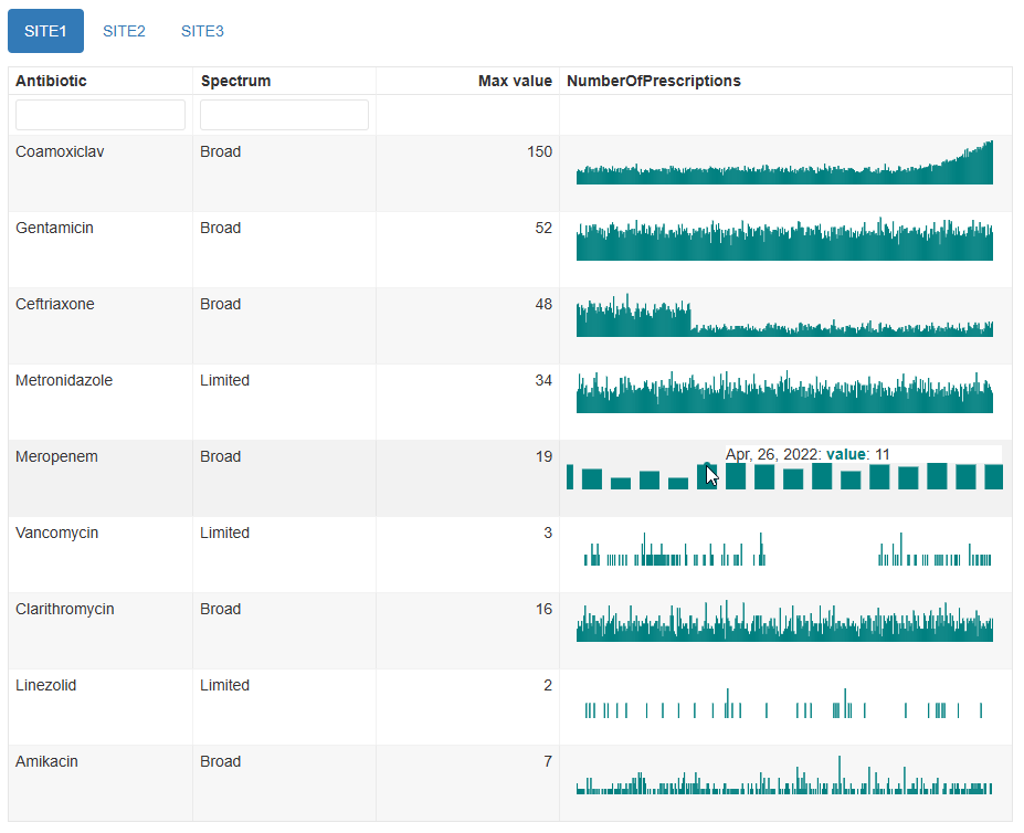
Interactive plots
This is the default visualisation, and produces a table with one time
series in each row, with orderable and filterable columns showing the
previously-specified item_cols for identifying the time
series. Also in the table are the maximum value of each time series, and
bar plots with adjustable axes and tooltips showing the individual dates
and values.
There are some options for adjusting the output, such as changing
column labels, plot type, and whether or not to use the same y-axis
scale across the table. This can be done using the
outputspec_interactive() function when supplying the
outputspec parameter.
Example:
For the example_prescription_numbers dataset above, we
will save a report in the working directory, with separate tabs for each
hospital site.
mantis_report(
  df = example_prescription_numbers,
  file = "example_prescription_numbers_interactive.html",
  inputspec = inspec_tabbed2,
  outputspec = outputspec_interactive(),
  report_title = "mantis report",
  dataset_description = "Antibiotic prescriptions by site",
  show_progress = TRUE
)
Static plots
Alternatively, the report can output static plots. This can be useful
if interactivity is not needed, or if file sizes need to be kept small.
There are currently two types of static visualisations: heatmap or
multipanel, and are selected by using the
outputspec_static_heatmap() or
outputspec_static_multipanel() function when supplying the
outputspec parameter.
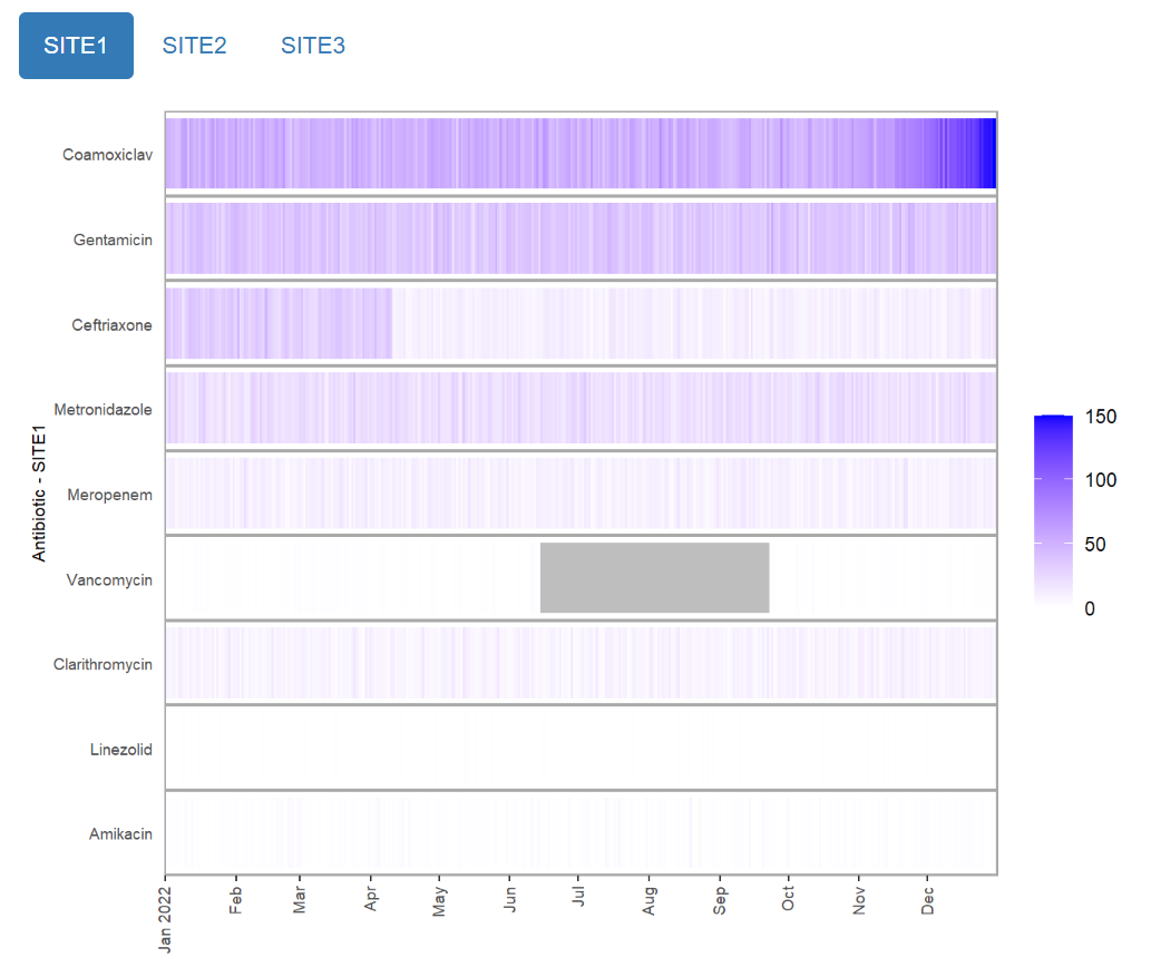
Heatmap
mantis_report(
  df = example_prescription_numbers,
  file = "example_prescription_numbers_heatmap.html",
  inputspec = inspec_tabbed,
  outputspec = outputspec_static_heatmap(),
  report_title = "mantis report",
  dataset_description = "Antibiotic prescriptions by site",
  show_progress = TRUE
)
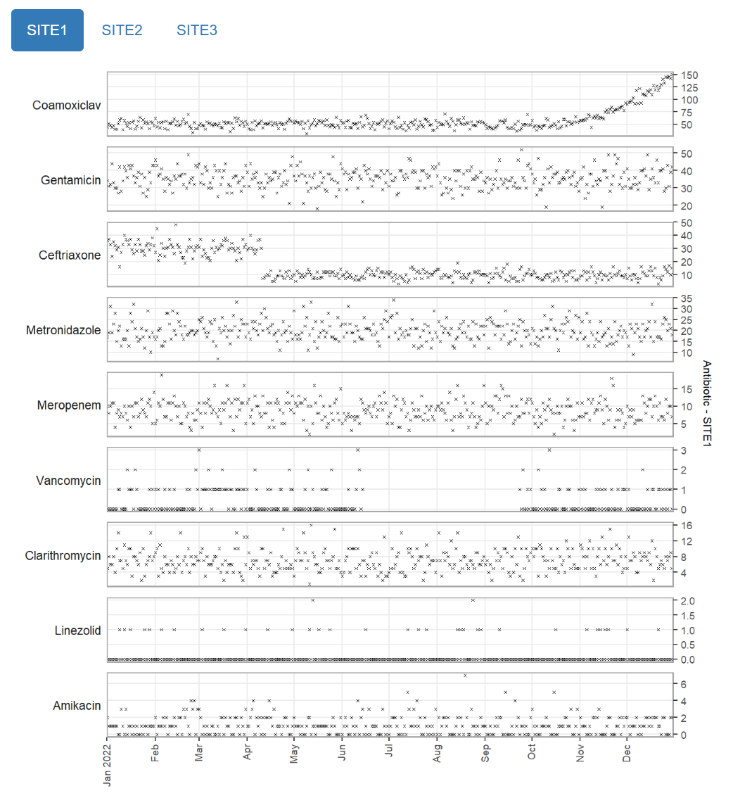
Multipanel
mantis_report(
  df = example_prescription_numbers,
  file = "example_prescription_numbers_multipanel.html",
  inputspec = inspec_tabbed,
  outputspec = outputspec_static_multipanel(),
  report_title = "mantis report",
  dataset_description = "Antibiotic prescriptions by site",
  show_progress = TRUE
)